
The author is an applied mathematician, not an expert in Photon Correlation Spectroscopy. Therefore, rather than present information about PCS, this document outlines the mathematical aspects of the "ill-posed problem" at hand and discusses a possible means to cure it. An overview of the algorithms implemented in DYNALS is provided, along with a description of how the algorithm's parameters may be changed through the DYNALS graphical interface. While using DYNALS, you will generally not need to alter computational parameters. However, this document includes recommendations regarding how and when these parameters may be altered to extract the maximum amount of information from your experimental data.
This document is neither a scientific paper nor a software manual. It is not rigid in the manner of a scientific paper and contains many practical tips and advices based on the author's personal experience. Unlike a software manual, it does not provide detailed step-by-step explanations of the DYNALS procedures, menu items, data formats, etc. This kind of information may generally be found in the DYNALS on-line help.
This document was last updated in March 2002
Appendix B. Tagged Data Format (TDF)
The coefficient G is related to the physical properties of the particles and the experimental conditions by the following expressions:
where
G is the decay rate
q is the scattering vector
DT is the translation diffusion coefficient
n is the refraction index
l is the scattered light wave length
Q is the scattering angle
T is the absolute temperature of the scattering solution
K is Boltzman's constant
h is the solvent viscosity
RH is the hydrodynamic radius.
In case of a poly-dispersed solution where the particles are not identical, the auto-correlation function of the scattered light intensity is described by the following pair of equations:

Disregarding the influence of inevitable experimental noise x(t) (discussed later), equation (2) allows us to compute the first order field correlation function g(1)(t) from the second order intensity auto-correlation function g(2)(t) accumulated by the correlator during the experiment.
DYNALS' treatment of the integral equation (3) will be the main subject of concern in the remainder of this document. This integral equation actually describes the relationship between the experimental data obtained during the experiment and the physical properties of the solution under study. If the decay rate distribution R(G) is known, then the Diffusion Coefficient Distribution or Particle Size Distribution can be easily computed using the equations (1). Sometimes the physical model may be more complex (e.g. if the particles are not spherical), in which case equations (1) must be replaced with something more complicated. The integral equation (3) forms the basis for data processing in Photon Correlation Spectroscopy.
This kind of equation with respect to R(G) is known as a "Fredholm integral equation of the first kind" and its solution is known to be an "ill-posed mathematical problem." Practically, this means that if the function g(1)(t) (experimental data) is known with even a minute error, the exact solution of the problem (the distribution R(G)) may not exist, or may be altogether different from the actual solution. On the other hand, the approximate solution is never unique. Within the experimental data error there exist an infinite number of entirely different distributions that fit the experimental data equally well. This does not mean that there is no reason to improve the accuracy of the experiment. The experimental error and the structure of the correlator (linear, logarithmic, etc.) define the class of distributions which may be used as candidates for the solution. The better the data, the smaller the number of distributions that fall within that class, thereby leaving fewer alternatives for the algorithm used to solve the problem.
Another method of reducing the number of possible solutions is to look only for non-negative solutions. Since a distribution can never be negative (i.e. the number of particles cannot be negative), this constraint is always valid and its use is always justified. Looking for non-negative solutions dramatically reduces the class of possible solutions and may sometimes even cause the problem to be stable. Generally, however, this is not sufficient. The class of non-negative distributions which fit the experimental data is still too wide to pick one of them at random and assume that it is close enough to the actual distribution. An additional strategy must be used to choose one particular distribution which will satisfy our intuitive notion about the physical measurements. Thus we must have some criterion that will allow us to express our preferences.
Generally, we would like to pick "the smoothest" distribution from the class of possible candidates. The difference between the various algorithms and their implementations is based on how this additional criterion is formulated and realized. In DYNALS, "the smoothest" distribution is quantified as the distribution with the smallest amount of energy, or for mathematicians, as the distribution of the minimal L2 norm.

The different approaches to the problem are discussed in the ensuing sections of this document.
If you are not familiar with the problem, now is a good time to try
out the DYNALS program and the included synthetic data sets.
This will give you a better feel for the problem and more importantly,
a deeper understanding of DYNALS and what you can and cannot
expect from the program. It is very important to play with synthetic data
as opposed to real data. In this way, you become familiar with the kind
of distribution achieved in the best possible scenario where no noise is
present in the data. You can observe how a higher noise level broadens
the class of possible solutions and how it influences the resolution achieved.
This will also help you attain the practical skills necessary to work with
DYNALS in your daily work. Initially, you are advised to
follow the instructions described in "Understanding
the term "ill-posed problem" in Appendix A.
The DYNALS on-line help, along with your own intuition, should be sufficient to help you begin the processing and enable you to obtain initial results. This document will help you interpret the results and make sure that information from the experimental data has been properly utilized.
DYNALS is under continuous development. Therefore, the operational instructions provided in this section may not be up-to-date. These instructions should provide you with tips and hints regarding the program's possibilities. Please refer to the on-line help for the exact names of menu items, entry fields and other details.
At the present time, DYNALS supports two data formats:
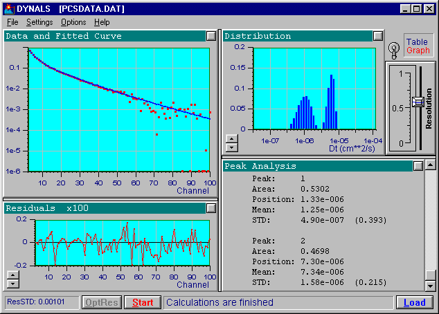
After the processing is completed, the DYNALS window appears similar to the one at the beginning of this document.
In the upper left part of the screen you will see the experimental data together with the fitted curve corresponding to the computed distribution. The lower left part of the screen shows the residual curve, which is the difference between the experimental data and the fitted curve. The residual curve is very important for estimating the quality of fit. For a good fit the residual curve should look random. If it does not look random either the data is 'underfitted', or there is a systematic error present in the data. In both cases the results are probably invalid.
The computed distribution is displayed in the upper right part of the screen and may be displayed as a graph or table depending on the position of the selection handle at the right. The distribution is computed using a logarithmic scale along the horizontal axis. The height of each column indicates the relative distribution area under this column which, due to the logarithmic scale, is not the same as its amplitude. The area under the entire histogram is normalized so that it is equal to one.
The lower right corner displays an analysis of the computed distribution. This window presents parameters of the entire distribution, its peaks and subpeaks. Note that the mean and the standard deviation of the entire distribution correspond to the values being computed and the method of cumulants. However, these values are generally computed more accurately by the distribution analysis.
You may use DYNALS without actually knowing what these terms mean. If this is the case, use the default distribution domain parameters and the number of distribution intervals larger than 50. If the residual values (bottom left window) look random, don't try to 'improve' the distribution by altering the resolution slider -- the distribution computed with the optimal resolution contains all the information that can be extracted from the experimental data. If you have absolutely reliable a priori information that your distribution consists of a small number (1 - 4) of very narrow peaks, you may try to set the maximum possible resolution by shifting the resolution slider to its upper position. This may dramatically improve the resolution due to the impact of the additional information you provided. Note, though, that if your information is incorrect, you will obtain a sharp but erroneous distribution. If the residual values do not look random then either you have a problem with your data (most probable), or the algorithm made a faulty estimation of the experimental noise. The following paragraphs explain how to verify this aspect of the distribution.
As mentioned above, the problem of computing the Particle Size Distribution from PCS data (or any related distribution) is an unstable, "ill-posed mathematical problem." The solution is not unique and generally should not be the one that provides the best possible fit for the experimental data in accordance with equation (2). Instead the solution should provide a reasonable fit which is stable enough. 'Reasonable fit' usually means 'up to the accuracy of experimental data. 'Stable enough means 'the one that does not change drastically with small changes in the experimental data. For example, we would expect to get similar distributions from several experiments made on the same sample although the data are slightly different due to inevitable experimental noise. When the random error in the experimental data increases, stability is improved by choosing a smoother distribution. In other words, the resolution decreases as the error increases.
The stability is always improved by reducing the number of degrees of freedom in the solution. The simplest way to reduce the number of degrees of freedom is to divide the distribution domain into a smaller number of intervals. For example, if you set the number of logarithmically spaced intervals as 10, this, together with non-negativity constraints on the solution, makes the problem mathematically stable. This kind of stabilization, sometimes called "naive" [2], constitutes the essence of the method of histogram [1]. Unfortunately, the approximation of the distribution of interest with only 10-12 intervals is too irregular. It thus prohibits the reconstruction of details which can be attained using more sophisticated algorithms. You may easily check this claim by setting the number of distribution intervals in DYNALS to 10 and shifting the resolution slider to its maximal value, thus effectively performing the method of histogram.
If the number of distribution intervals is large enough (recommended value is 50 or larger), the resolution slider position shows the trade-off between the fit of experimental data and the maximum attainable resolution. It should be understood that resolution along the G axis is not constant. It varies for different values of G and depends on the accuracy of experimental data, the structure of the correlator and on the distribution itself. For example, with good authentic data, it is possible to resolve two delta functions d(G- G1), d(G- G2) (two peaks) with G2 / G1 =3 when they are in optimal position on the G axis (about the middle of the default distribution domain) Footnote 2 . The same resolution (3:1) is not possible if delta functions are located closer to the DYNALS default domain ends or if additional components are present in the distribution. You may learn more about the resolution and its dependence on the above factors by practicing the exercises "Understanding the resolution and its dependencies" in Appendix A.
If the resolution slider value is too low, the distribution will not have enough detail to provide a good fit for the experimental data. If the value of the resolution slider is too high, the data will be "overfitted", where the details of the distribution may not be reliable due to the noise in the experimental data. The optimum value is in between, so that the resolution slider value is the smallest one that provides a good fit. The stabilization algorithm implemented in DYNALS automatically finds and sets this optimum value.
In general, you will not need to alter the optimal resolution slider value once it has been set after new experimental data has been processed for the first time. Whether your data are real or simulated with a reasonable noise, you will always get a value between 0 and 1 for resolution slider.
There are three cases where you might want to alter the optimal resolution value:
Let us begin with the solution to the integral equation (3). The document will present a numerical analysis of the problem (3) in the discretized form and explain why this problem stands as one of the most severe inverse problems in applied mathematics. This section investigates the corresponding system of linear equations and how the properties of the matrix are reflected in the solution. The traditional approaches to the problem are discussed, both the ones which are specific to the equation (3) and the ones having the equation (3) as a particular case. An introduction to the algorithms implemented in DYNALS is then presented, in order to give you an understanding of why these algorithms are superior to the traditional ones. The section also discusses possible improvements which may be implemented in future versions of DYNALS. At the end of this section, the author briefly reviews the complications caused by using the second order correlation function g(2)(t) accumulated by the correlator to compute the field correlation function g(1)(t) used in the equation (3).
First of all, the correlation function g(1)(t) is known only on a limited set of points {ti}, i=1,M , where M is the number of correlator channels. (The problem of computing g(1)(t) from g(2)(t) is discussed later). The set is defined by the particular correlator structure in use. This structure may or may not be uniform. This discretization of equation (3) leads us to the following system of equations:

where xi are the noise values, and the integration boundaries of equation (3) are replaced with [Gmin,Gmax]. The replacement of the integration boundaries reflects the loss of information caused by the finite correlation time ranges covered by the correlator channels. Indeed, the small values of G correspond to slow decays of the correlation function so that Gmin can always be chosen small enough, such that if G< Gmin then exp(-Gti) is indistinguishable from a straight line (and hence from each other) due to the errors xi . On the other hand, large values of G correspond to fast decays of the correlation function. Due to a finite value of t1 , there always exists a value Gmax such that if G> Gmax then exp(-Gti) falls below the noise level before the first channel. The idea is illustrated by the following figure:
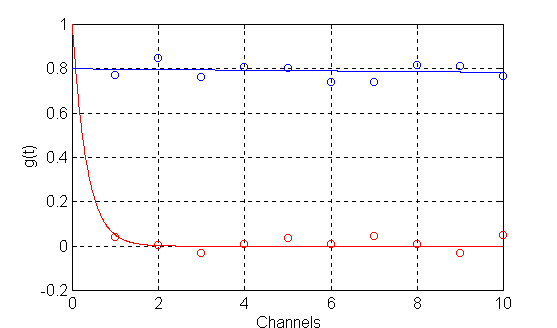
It is clear that while using only the measured values {g(1)(ti)}, i=1,10 it is impossible to distinguish the blue curve from the constant and the red curve from zero. In DYNALS, the default range for G is set as [Gmin=0.1/tM , Gmax=5/t1] so that it is wide enough to cover the maximal possible range for even the smallest possible noise in the correlator channels.
Having the set of equations (4), the next step is to find a parametric representation for P(G) that is both non-restrictive and allows the use of an effective numerical algorithm. Various representations have been proposed which lead to different reconstruction methods. For example, using the first cumulants of P(G) leads to the method of cumulants [3,4]. Using a parametric distribution of particular shape (or their superposition) with unknown parameters leads to a nonlinear fitting procedure. Examples include several delta functions for multi-exponential fit, Gaussians [5], Pirson distribution [6], log normal distribution [7] and some others. Specifying the distribution as a number of a priori spaced delta functions leads to the exponential sampling method [5] when the number of delta functions is small, or to regularization methods [2] like the one used in CONTIN [8,9] when this number is large. When the distribution is approximated by a relatively small number of histogram columns (10-12) with specified boundaries, the method is called "the method of histogram" [10,11]. A short survey of the methods appears in Section 3.3.
In DYNALS, as in the method of histograms, the distribution in the range [Gmin, Gmax] is also approximated by a number of rectangular columns. The columns are adjacent to each other, where the column boundaries are spaced using the logarithmic scale substantiated by the behavior of the eigen functions of equation (3) [12,13]. Denoting the boundaries of N columns as { Gi } where i=0..N, Go=Gmin , GN=Gmax leads to the system of M linear equations with N unknown coefficients {xi}

or in a compact form:

The difference between the discretization in DYNALS and in the method of histogram is in the number of histogram columns used to represent the distribution. In the method of histogram, the stabilization of the problem is achieved by reducing the number of columns N to about 10-15. Using a small number of columns to approximate the distribution of interest leads to a very coarse distribution with pure resolution and appearance. In DYNALS, the stabilization is achieved by using the developed, proprietary method for solving the above system of equations while constraining the solution to remain non-negative. Additionally, special scaling for columns of the system matrix A, together with the solution of the minimal norm ||x|| leads to the computation of the distribution P(G) having the smallest L2 norm (or energy in physical terms) that is:

Numerous computer experiments have shown this property to be very useful for proper reconstruction of the distribution of interest.
Another important factor that must be taken into account is that errors in the elements of the vector g are unequal (see Section 3.5). Numerically it is accomplished by replacing the original system (6) with the weighted system Awx=gw , where Aw=WA, gw=Wg and W is the diagonal matrix with elements wii =1/si inversely proportional to the standard deviation of the corresponding values gi. To keep the notations simple, the superscripts denoting weighting will be omitted in the following sections. However, it should be noted that the weighted system of linear equations is always used in the actual computations made by DYNALS.
We will use Singular Value Decomposition (SVD) as the main analyzing tool. The singular value decomposition of a rectangular, mxn matrix A is defined as A=USVT , where U and V are orthogonal matrices and S is a diagonal matrix [14] with non-negative elements. An orthogonal matrix is a matrix whose transposed matrix is equal to its inverse i.e. UUT= UTU=I where I is the identity matrix. They have the remarkable property that ||Ux||=||UTx||=||x|| i.e. multiplying a vector by an orthogonal matrix does not change the vector's length. This property is very important since it allows us to characterize such matrices as "good" matrices; if we have a system of linear equations Ux=g, the solution of the system is trivial x=U-1g= UTg (see the definition of orthogonal matrix above). When =g'+dg , where dg designates an error component in the right hand side, the solution vector is composed from two components x=x'+dx=UTg+UTdg. When ||x||=|| UTg||=||g|| and ||dx||=||UTdg||=||dg|| , it follows that ||dx||/||x||=||db||/||b|| is the relative error in the solution and is always equal to the relative error in the data. A better solution is unavailable without additional information.
Unfortunately, the properties of the system matrix A are defined by the diagonal matrix S, which in our case is a problematic matrix. Let us make some transformations of the original system of linear equations (6) to see what is so problematic in this very simple, diagonal matrix S. Replacing the matrix A with its singular decomposition gives us the system USVTx=g. Multiplying the right side of this system by UT results in SVTx=UTg (see the definition of the orthogonal matrix). By making simple changes in the variables p=VTx, f=UTg we get a new system of equations Sp=f .
Recalling that the matrix S is diagonal, the solution of this system may seem to be trivial p=S-1f=[f1/s1,f2/s2,.. fN/sN]T . Unfortunately, our case is not that simple. If the right side of the initial equation is known with an error dg, then f=f'+df where df=UTdg, and in accordance with the property of orthogonal matrices above, ||df||=||db||. Due to the error dg, using the same property, the error in the solution p is dp= S-1df and ||dp||=||dx||. It is now apparent that the sensitivity of the solution to errors in the data is defined exclusively by the matrix S. The diagonal elements of matrix S are called the singular numbers of matrix A, and their properties resemble the properties of the singular numbers of the functional operator (3). It may be shown that:
where c(A) is known as the "matrix condition number". This equation states that the relative error in the solution vector is proportional to the relative error in the data vector and the condition number of the system matrix. When the ratio of the two extreme singular numbers is small, the matrix (and the problem) is termed "well-conditioned". The best possible case is, obviously, c(A)=1 which corresponds to orthogonal matrixes. When the ratio of the two extreme numbers is large, the matrix (and the system of linear equations) is termed "ill-conditioned" which resembles the term "ill-posed" used to describe the parent, continuous integral equation (3). When the minimal singular number is zero (they are always non-negative), the matrix and the system of equations are called "singular".
In our case, the singular numbers of the system matrix A decay to zero very quickly, thus complicating the problem. The following figure illustrates the decay of singular numbers for three cases:
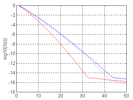
The leftmost, red solid line shows the logarithm of the singular numbers for uniform distributed data points {ti=Dt*i}, i=1, M, where M=100, Dt=1 and [Gmin=0.002, Gmax=5]. The blue line corresponds to the same conditions but for M=500. Enlarging the number of correlator channels alleviates the problem, however the improvement is not dramatic and does not transform the problem into a "well-behaved" one. It does extend the possible reconstruction range towards smaller gammas in proportion to the number of channels (to Gmin=0.0004 in this case). The same effect may be achieved using a much smaller number of logarithmically distributed channels covering the same range (1 - 500). The magenta dashed line shows the singular numbers for M=50 and { ti= ti-1+max( floor(exp(i*q)), 1) }, i=2, M , t1=1 and the constant q is chosen for tM=500.
The singular numbers decay so fast that they drop below the single precision computer arithmetic somewhere around the 20th singular number and below the level 10-3 corresponding to a suitable accuracy in the correlation function just after the tenth number. If we recall the relation (7), we understand why the maximal number of histogram columns cannot be larger than 12. The relative errors in the histogram's column heights become so large that they are unacceptable.
In the first category, only a small number of unknown coefficients are used to describe the distribution of interest. The singular numbers of this impaired problem do not have a chance to decay too much (see Figure 2) and therefore the problem remains stable. In the second category, the singular numbers are modified (direct or indirectly) so they suppress the subversive influence of the inverted small singular numbers. The following sections briefly review some of the most widely used members of both categories, where section numbers describing the first category use the numbers An, and section numbers describing the second category use the numbers Bn.
where {mi} are the central moments of the distribution of interest P(G). The average gamma value is equal to the first moment, and its standard deviation is given by the square root of the second moment. The third moment theoretically describes the asymmetry of the distribution. The other coefficients are more difficult to interpret.
The coefficients {mi} may be easily found by solving the corresponding system of linear equations. Stabilization is achieved by reducing the number of unknown coefficients used to approximate ln(g(1)(t)). Generally, only the first two moments (and thus the average and the dispersion) can be reliably reconstructed. This provides very limited information for multi-component distributions or when dust is present.
The method of histogram has the following two drawbacks. Firstly, the maximum number of histogram columns which can be reliably reconstructed is not constant. Another drawback is that the logarithmic resolution is not optimal. Both the number of histogram columns and the optimal resolution law depend on the reconstruction range, the structure of the correlator in use, the noise in the experimental data and the distribution of interest itself. This dependence is not simple, and may be taken into account by using the singular value decomposition of the system (6).
The advantage to using the singular value decomposition over other methods of solving the system of linear equations is that it allows us to easily remedy the solution to some extent by extracting only the stable or reliable information. This is done by replacing the matrix S-1 in the above equation with the matrix S+=[1/s1,1/s2, ,1/sK,0,...,0]T where the singular numbers should be sorted in descending order, sK/s1>x and sK+1/s1<x . If we make a simple change of variables p=VTx, f=UTg and recall the properties of orthogonal matrices, the idea of remedying the problem with Singular Value Decomposition may be easily understood:
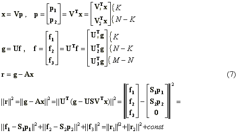
where ||r|| is the residual norm, which is minimized in the method of least squares. If M>N, the last term is constant and cannot be minimized, no matter which method is chosen to solve the system of equations. In the method of truncated singular value decomposition, the second term ||r2||2 is not minimized either. Recalling the definition of the matrix S+ above, it leads to setting p2 to zero, ||r2||=||f2|| and ||r||2= ||r2||2+const. The hope is that sacrificing the residual norm to some extent, we can find a solution which is less sensitive to errors in the vector g. The idea may be more clearly presented if we use the property of orthogonal matrices ||x||=|| VTp|| and write the full expressions for the residual and the solution norms:

where as before, f'=UTg' and df=UTdg denote the transformed exact data and the error vectors respectively. It can be seen that incrementing K leads to the reduction of the squared residual norm on the quantity fK2 and the enlargement of the squared solution norm on the quantity (pK/sK)2. Using functional analysis it may be shown that without the error term df, the coefficients {fi} decay to zero and thereby compensating for the influence of the small singular numbers. The errors {dfi}, divided by small singular numbers, introduce large, wild, components into the solution, making it totally inappropriate. The art of using the truncated singular value decomposition is to find a compromise (an appropriate K) between the residual and solution norms, keeping them both relatively small. Generally, if some freedom is allowed in the residual norm, there exist an infinite number of solutions possessing the same residual norm. It is important to note that of all these solutions, the solution computed by the truncated SVD possesses the smallest Euclidean norm.
The good news for users of truncated SVD is that the appropriate value for the component K can almost always be found. The bad news is that in our particular case its value is too small. Without using any other a priori information, this number is generally limited to 4 - 6 values which gives a very rough solution. Worse than that, if the distribution of interest is computed in a relatively wide range [Gmin,Gmax], it will have large oscillating or negative tails which have nothing to do with the true distribution. Additional information is necessary to make the method of truncated SVD useful. Different attempts have been made to impose auxiliary constraints on the solution, but, prior to the development of the unique algorithms implemented in DYNALS, no adequate solution suitable for commercial use was found. In these algorithms, the truncated singular value decomposition is combined with non-negativity constraints on the solution. This eliminates oscillation and negative tails and allows numerical analysis of the vector f so that the number K can be chosen automatically.
In Tikhonov's method of regularization for the continuous case, the corresponding system of normal equations is used to find the unknown coefficients. The system is derived from the system of linear equations (6) by multiplying its left side by the matrix AT as Fx=b , where F=ATA and b=ATg . The exact solution of such a system minimizing the norm ||Fx-b|| is equivalent to the least squares solution of system (6), and is therefore unstable. To make it stable, the initial expression for the norm to be minimized is replaced as follows:
where the term ||G||2, called the regularizer, defines the additional properties in favor of which we are ready to sacrifice the best possible fit. For example, if we would like to minimize the solution norm, we can set G=I, where I is the identity matrix. Most often, the matrix G encompasses a value associated with a 'smooth' solution. For example, this value may be the first or second derivative operator or its combination with the identity matrix. The coefficient a, called the regularization parameter, allows us to define the strength of the constraint on the solution. Very small numbers or zero do not introduce a constraint, and as a result the computed solution is unstable and has little in common with the actual solution. On the other hand, numbers that are too large pay little attention to the data, resulting in a solution that is smooth and nice but 'underfits' the data and hence extracts only part of the information available in the experimental data.
Technically, the method is implemented by using the modified system of normal equations devised as follows:
Applying the singular value decomposition, it may be shown that using the solution norm as the regularizer (G=I) is equivalent to replacing the singular numbers with si'=(si2+a)1/2. Such substitution alleviates the problems associated with small si by damping large elements of S+ in accordance with the formula:

Other regularizers provide different damping factors but employ a similar idea - they all decay smoothly towards zero as the corresponding index i increases. Alternatively, the solution computed by the truncated singular value decomposition may be associated with the damping factors computed as:

where h is some threshold value. The proper choice for h is discussed in the following section devoted to the algorithms implemented in DYNALS.
In our case, there are two major difficulties associated with the method of regularization. The first one is related to the fact that the singular numbers decay very fast while the damping factors decay slowly. If a is chosen to damp all problematic singular numbers, it will partially damp the stable ones and, therefore, not all available information will be extracted from the data. On the other hand, if a is chosen to pass all valuable information, it will also allow small singular numbers to ruin the solution. The value in the middle will partially damp the stable information and partially pass the amplified noise (by dividing it into small singular numbers) and, as a result, the optimal solution is never found. A large number of published papers have been devoted to the optimal choice of the regularizer and the regularization parameter. Most, if not all of them, assume that the problem is linear, which in our case greatly underestimates the regularization parameter. The reason for such underestimation is that the system of equations is to be solved under the constraint of a non-negative solution. This constraint greatly improves the stability of the problem but causes the problem to be nonlinear (by the definition of a linear problem) and the corresponding, "optimal" a to become irrelevant.

where all the vectors and matrices are defined in equations (7) above. The expression (11) for minimization of the norm may seem to resemble the expression (8) minimized in the method of regularization (Section B2 above). However, in (11) different vectors, p1 and p2, are used in the two terms of the minimized function. The first vector, p1, is used to provide the minimal residual norm using only those stable components of the singular value decomposition corresponding to the large singular numbers. The second vector, p2, is used only to make the solution vector x non-negative. If the solution x, provided by unconstrained minimization of ||f1S1p1||, is non-negative (or the constraint (12) is not applied), then nothing prevents p2 from being equal to zero and the solution is equivalent to the truncated singular value decomposition. Otherwise, the vector p2 is not zero and its components manifest additional information introduced by the non-negativity constraint. In other words, the vector p2 serves to give freedom to the vector p1, such that some tradeoff between the minimal truncated residual norm ||f1-S1p1|| and minimal truncated solution norm ||p2|| is reached. The tradeoff depends on the parameter b as follows: If b is too large, the second term ||p2|| is excessively constrained and does not provide enough freedom to the vector p1 (due to the non-negativity constraint) and the solution underfits the data. On the other hand, if b is too small, the vector p2 may take on wild values just to satisfy the constraint (12). The optimal value is found to be directly proportional to the accuracy of the experimental data, the maximal singular number and the norm ||f1||. The explanation of such proportionality is beyond the scope of this document.
Technically, the problem of minimizing (11) under the constraints (12) is solved by transforming the problem into the equivalent LDP (Least Distance Programming) problem, which is then solved by the method described in [16].
To implement the equations (7,11,12), we must divide the set of singular numbers into two subsets, the subset K "big" numbers and the subset N-K "small" numbers. If the input data were perfect, we might regard all the singular numbers as "big" so that K would be equal to N Footnote3. When noise is present, this type of solution will be unstable. Therefore, the size of the first subset must depend on the accuracy of the experimental data. On the other hand, the relative influence of the random noise on the elements of f is also different. The vector f may be rewritten as f=f'+df=UTg'+UTdg . It can be shown that the elements of f' rapidly decay to zero while the standard deviation of the elements df remains the same (orthogonal transform of a random vector). It seems reasonable to minimize the residual norm using only those elements of f which significantly exceed the standard deviation of the elements df . With this choice, the size of the subset for "big" singular numbers depends not only on the noise in the experimental data, but on the distribution of interest itself. This is reasonable since a smaller number of singular value decomposition components are necessary to approximate a "smooth" distribution than to approximate a "sharp" one.
In DYNALS, the tail of the vector f=UTg is used to find sn (the standard deviation of the noise). After that, the noise level is set as 3sn and only those elements of f that are larger than this level are used for residual norm minimization. The actual implementation is a bit trickier when coping with the different complications caused by unusual noise statistics or non-random noise (systematic error), but the idea is the same.
is associated with certain complications. First of all, for large values
of t, the expression under the square root sign may be negative. In this
case, calculating g(1)(t) requires computing the
square root of a negative number. The standard procedure used in photon-correlation
spectroscopy uses the trick of setting ![]() ; this is reasonable, but odd from a purely mathematical point of view.
Actually, using complex numbers does not eliminate the problem's difficulty.
The function g(1)(t) is real and the imaginary
parts must be dropped for further processing. This is equivalent to setting
; this is reasonable, but odd from a purely mathematical point of view.
Actually, using complex numbers does not eliminate the problem's difficulty.
The function g(1)(t) is real and the imaginary
parts must be dropped for further processing. This is equivalent to setting ![]() which is worse than the standard rule and leads to larger systematic errors
in the values of g(1)(t).
which is worse than the standard rule and leads to larger systematic errors
in the values of g(1)(t).
[17] shows that even when the value under the radical is non-negative, calculating g(1)(t) from (13) increases the random error (relative to g(2)(t)) and introduces a systematic error. [17] also proposes to compute the distribution of interest in two stages. In the first stage, the self-convolution of the distribution of interest R(G)* R(G) is computed from the function g(2)(t)1. The smoothed estimation of g(2)(t) is then computed and used to compute the first order correlation function g(1)(t). Computer experiments have shown that this type of two stage processing provides better resolution. The option of two stage processing will be implemented in a future version of DYNALS.
In the meantime, weighting is used to alleviate the problems described above. Every row i of the matrix A in (6) and every element i of the data vector g are multiplied by the corresponding weight wi . The weights are set in accordance with [18] as:

providing good results (giving a random residual vector) in most cases.
All exercises are performed on synthetic data, which has two main advantages. Firstly, you know the true distribution in advance, which is very important when you are trying to understand the character of distortions caused by the stabilization procedure. Secondly, synthetic experimental data do not contain systematic error. Systematic error is generally very difficult to separate from data, and sometimes leads to the unpredictable distortion of results.
There is a variety of different synthetic data provided with DYNALS, along with a complete list describing the files. Several files, corresponding to different experimental noise levels, are provided for each distribution. It is supposed that the noise is normally distributed and uncorrelated between the channels. The last four numbers in the name of every file indicate the standard deviation of the error. For example, files 'xxxx0000' correspond to precise data, files 'xxxx0010' correspond to the standard deviation 0.001, etc. Files whose name begins with 'u', correspond to the uniform 100 channel correlator and a sampling time of 1 microsecond. Files whose name begins with 'l', correspond to the 50 channel logarithmic correlator and the same sampling time. You can look at the files to see how the channels are distributed.
The exercises may be performed using any distribution units (decay rates,
decay times, diffusion coefficients or hydrodynamic radii), however we
recommend using decay rates. The screen shots provided below correspond
to decay rates in megahertz.
In this exercise we use a wide, unimodal distribution. Load the file up1w0000.tdf corresponding to the accurate data and click the Start button. After the processing has finished, you will see the following distribution which is the true one.
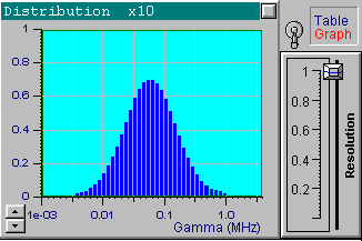
Note that DYNALS sets the maximal possible resolution since the data are considered perfect. It does not mean that there is no stabilization; a minimal stabilization is used to compensate for finite computer arithmetic precision.
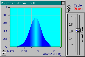
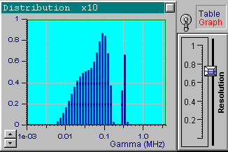
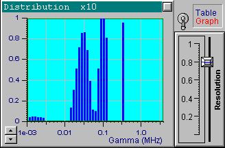
We will now choose another data set from the file up1w0010.tdf, which corresponds to the same distribution but includes noisy data. As indicated by the filename, the noise standard deviation for this file is 0.001. Click the Start button to receive the first in the following series of four pictures. These pictures correspond to the optimal resolution that is automatically set by DYNALS. The corresponding residuals are random, i.e., this distribution provides a good fit for experimental data. The position of resolution slider leaves you some freedom to experiment. By increasing the resolution slider value you can see that the shape of the distribution changes dramatically, while the residuals actually stay the same. The other three pictures provide examples corresponding to three different positions of the resolution slider. Each of these four distributions, along with an infinite number of the others corresponding to values of the resolution slider larger than the optimal one, provide a good fit to the data. Try using values that are less then optimal. You will see that the distribution computed using smaller resolution slider values does not provide a good fit.
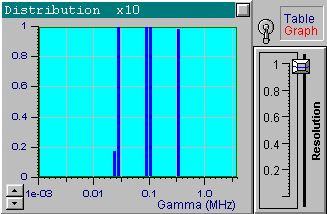
Now load the file up1w0030.tdf, which corresponds to the same
distribution but has more noise. After processing the data, you will see
that the optimal resolution value is around 0.5. This value is lower than
the one used for the previous file, which reflects the fact that the data
is less accurate and more freedom is left for the solution. Try changing
the position of the resolution slider to see a variety of the possible
solutions.
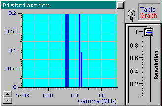
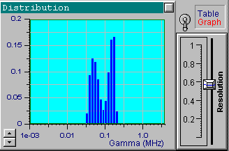
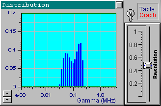
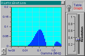
It is clear that the resolution decreases as the noise increases. Note how the resolution slider reflects the accuracy of experimental data. You can see a small separate peak in the last picture (the most noisy data). This peak corresponds to very fast exponentials which do not actually exist. Its presence is explained by the large noise in the first one or two channels which is confused with very fast decaying components. There is nothing we can do with it, except perhaps to avoid fitting the first channels for very noisy data. Try it. It helps in this case. You can also try using the a priori information that the distribution of interest consists of narrow peaks. By setting the maximal value of the resolution slider, you will get the same sharp distribution shown in the first picture. Be careful with this approach though, for a relatively large noise and a multi-component distribution you may get incorrect peak positions.
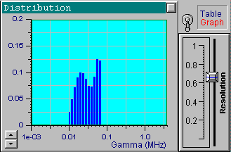
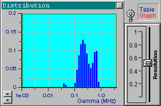
As you can see, the peaks are less resolved than when located in the optimal resolution region. If the reconstruction region is defined automatically, this region is always located in the middle of the plot, which may serve as a good hint for a proper choice of the sampling time. If the decay rates or the diffusion coefficients are set as the reconstruction units, then reducing the sampling time corresponds to the distribution being shifted to the left (exponentials decay slower). Increasing the sampling time accelerates the decay and the distribution moves to the right. If the decay times or hydrodynamic radii are used, then the opposite is true.
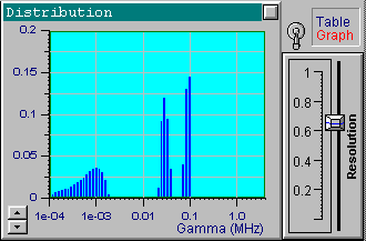
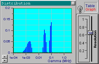
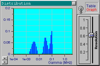
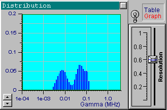
It is obvious that the resolution depends on the distribution itself.
The algorithm implemented in DYNALS makes a special analysis
of experimental data and chooses the optimal (i.e. the maximal possible)
resolution when no extra, a priori information is available.
[PCSPHYSPAR]
WAVELENGTH= 632.8
VISCOSITY= 1.0
SCATANGLE= 90.0
TEMPERATURE= 293.0
REFRINDEX= 1.33
[PCSDATA2]
1= 1.000000e-006 1.760349e+000
2= 2.000000e-006 1.596440e+000
3= 3.000000e-006 1.480216e+000
. . . . . . . . . . . . . . . .
99= 9.900000e-005 1.001706e+000
100= 1.000000e-004 1.002411e+000
The brackets are part of the syntax. The order of the sections and the tags inside the sections is arbitrary. The following section names are recognized by DYNALS :
[PCSDATA2] -- for the second order (intensity fluctuations) auto-correlation function measured under the homodyne scheme. The section's tags define the numbers of corresponding correlator channels. The information field consists of two numbers: time delay (in seconds) corresponding to the particular channel and the normalized correlation function value in that channel.
[PCSPHYSPAR] -- physical parameters of the experiment where the data were acquired. The following tags are recognized in this section: